

Successful management of California’s freshwater resources requires balancing consumptive and non-consumptive water use with fish species that depend critically on the same resources. Numerous water management decisions are being evaluated currently, many with the goal of protecting endangered species such as winter-run Chinook salmon. Scientists at UC Santa Cruz, NOAA Fisheries, USGS, and QEDA Consulting have developed a winter-run life cycle model to support such decision-making in the Central Valley.
The winter-run life cycle model can incorporate other models that run at finer spatial and temporal scales, such as SALMOD, and has been statistically fitted to winter-run abundance data from multiple life stages. The winter-run life cycle model has been applied in several important decisions, such as evaluating long-term operational scenarios, Shasta temperature management, and defining how restoration and associated survival experiments can increase the productivity of the winter-run population.
At the 2021 Bay-Delta Science Conference, Dr. Noble Hendrix, Biometrician at QEDA Consulting, gave a presentation on how the winter-run life cycle model has been used to aid decision making for managing winter-run salmon. Ann-Marie Osterback at UCSC, and Eric Danner and Evan Sawyer at NOAA are colleagues in this work and presentation.
 The need for the winter-run life cycle model stems from wanting to understand the decline and the change in the population abundance, shown here from the 1970s. The winter-run chinook salmon were initially listed in 1989 and identified as endangered in 1994. In 2009, before the development of the model, a biological opinion written for the long-term operations of the Central Valley Project and State Water Project came to a jeopardy opinion, which was subsequently challenged in court.
Judge Oliver Wanger, the presiding judge, wrote in his ruling, “… this is the last time NMFS will be permitted to avoid studying, analyzing, and applying a life cycle model. NMFS‘s chronic failure to do so now approaches bad faith in view of the undeniable importance of the information to resolve the perennial dispute over population dynamics. At some point, this diminishes the agency‘s credibility.”
“What he was getting to is the underlying value of the life cycle models for trying to answer important questions,” said Dr. Hendrix. “Aspects of life cycle models that make them useful for answering these types of operational or other questions are that they integrate across individual models or individual life stages to understand what the effects are on the population. In addition, multiple environmental conditions are also integrated across, such as different water year types.”
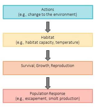 “They also provide a nice framework for connecting mechanisms that affect life stages of the winter-run (or other species) being modeled,” he continued. “There are factors that affect those life stages, and then there are management actions that then affect those factors. So it creates a nice linkage between the actions that are being evaluated and the ultimate impacts on the population. And for that, they are really useful for these types of analyses of looking at hydromanagement questions.”
The winter-run life cycle model can address a suite of different questions; this presentation will discuss the questions around restoration and management actions around temperature and reintroduction. He noted other uses for the model include evaluating water operations scenarios, data gaps, real-time management, and adaptive management approaches.
The life cycle of winter-run chinook salmon, like all salmon runs, has an egg to fry transition; rearing among different habitats, such as the upper river, lower river, floodplain, and Delta habitat; coming down through the Bay, undergoing smoltification in the smolt stage, and then out-migration, past the Golden Gate into the Gulf of the Farallones, and to the ocean. Adult salmon can return as 2, 3, or 4-year spawners which return to produce eggs.

The geographic or spatial domain is the Upper Sacramento River, from Keswick Dam and the Red Bluff Diversion Dam to Sacramento and the Delta, the Bay, and the ocean.
The transitions in the life cycle model are defined by equations. He said the equation for the egg to fry survival is somewhat complicated. “We have a baseline survival that’s applied if we’re below a critical temperature, in this case, 13.5-degrees C. And there’s a relationship that’s applied when you’re at a temperature above that critical temperature. In this case, there’s an exponential decline in the survival rate, as the temperatures go higher and higher above the 13.5-degree temperature threshold.”


Each transition has an underlying mathematical equation or an underlying model, which is a group of equations. The ability to incorporate other models that may be specific for given life stages into the overall framework of the life cycle model gives it flexibility. For example, the smolt survival during migration from rearing to the Gulf of the Farallones is calculated by running a separate EPTM version two model, which can reflect dynamics at a much finer spatial and temporal scale.
 So, to make this particular model structure (somewhat generic) apply to winter-run, the model must be fit to winter-run estimates of abundance.
“This works by having mathematical relationships that are composed of coefficients and then estimating those coefficients by using observed data from the winter run populations,” said Dr. Hendrix. “We have spawners below Keswick, we have juveniles collected at Red Bluff diversion dam, we have juveniles collected in Knights Landing catches and rotary screw traps, and then we have estimates of Chipps Island abundance. All of these form a time series of abundance estimates.”
The abundance data is fitted to the model using a statistical approach, as shown on the chart below. The model predictions are shown in red, the observed data are shown in black, and the dashed lines are the measurement error around those observations.

“So in fitting to the data, we can then basically have a model that’s reflecting the historical patterns and abundance for winter-run,” said Dr. Hendrix. “Then we can use that model for making evaluations of different management alternatives.”
Using the life cycle model to evaluate restoration options
 One application of the model is to evaluate restoration projects: Which should we restore: upper river, lower river, Yolo Bypass, or Delta?
“We’re not really sure what the overall survival benefits are of doing that restoration,” said Dr. Hendrix. “We do know that high-quality habitat (which we assume we would restore to) can improve the growth rates, and therefore the size of the individuals. But we’re not sure exactly how that translates into those individuals of a larger size surviving at a higher rate.”
Three different levels of survival benefit are assumed: 0% or no difference, 5%, or 10% benefit to rearing in high-quality habitat. This information is then used to try and understand which of these areas should be restored.
 “We run the lifecycle model and what we obtain is an estimate of the number of spawners, according to the model, under 0% survival benefit by restoring the upper river with 500 acres of high-quality habitat,” he explained. “Likewise, we can do this for the lower river and the Yolo. And we can obtain these estimates through the model of spawner abundances for each one of these combinations. Because we don’t know which of these survival rates is true, we average across all of them for each one of these actions. So we can see that the action that provides the highest average benefit is restoring the lower river. And that gives us 10,610 modeled fish in year 45.”
If the scenario is changed so that we do know what the survival benefit is, then we can also go back to the matrix and ask a slightly different question, which is, if we knew that the survival rate was 0%, what action would we do?
 “We would restore the Delta because that’s the one that provides us the biggest benefit if the true survival rates 0%, he said. “Likewise, if we knew the survival rate was 5%, then we would restore the lower river. If we knew it was 10%, we would restore the lower river again, so if we average these values, we get 11,177 spawners. And so by knowing survival, we can get 5% more (11,177) spawners than without knowing survival (10,610).”
“What this calculates is the expected value of knowing what the survival benefits are when in fact, we don’t. We still don’t know what they are, but we can do monitoring to understand what the likely value is. And so this EVPI, or the expected value of perfect information, sets an upper bound on the value of doing this monitoring. A 5% increase in the population due to doing restoration actions would be considered a moderate improvement. And so that would, that would suggest that monitoring is an important step relative to the restoration actions.”
Shasta temperature management
 The second example is understanding how temperature management at Shasta could potentially improve the population dynamics and the benefits of reintroducing fish above Shasta Dam.
Dr. Hendrix said there are a couple of specific actions for changing or modifying the temperature profile.
The first action is to reduce the temperatures during the peak spawning months of June and July; the trade-off is increasing temperatures by one degree C during May and August. The second action is to trade a cooler temperature in April for a warmer temperature in September. What would be the effect if those actions were taken in all years versus just the critically dry years?
Another related question is what would be the effect of reintroducing winter-run above Shasta Dam in only the strongest critical years when conditions are very hot and dry versus doing that in all years?
The reintroduction is implemented in the model by collecting spawners that are then placed above Shasta Dam in the McCloud and Sacramento Rivers. The juveniles produced through spawning are collected at the head of the reservoir and transferred down to below Keswick Dam, where they enter the model either as fry or smolts. The proportions are about 5% going to the McCloud River and 1% to the Upper Sacramento River.
 “For the results, basically we see a positive effect in this peak for shoulders, and that’s mostly happening due to critical years,” said Dr. Hendrix. “When we do a reintroduction on top of that, we see a synergistic net benefit, so an improvement over just adding the two together. However, essentially the April through September approach is negative in all cases, suggesting that that would not be a good approach for doing temperature management.”
QUESTIONS & ANSWERS
QUESTION: Do you know if the values you estimate by survival rates are actually statistically different from one another?
Dr. Hendrix: “We can look at the way the model is structured, so we can structure the model and basically allow certain parameters to be estimated versus not estimated. We can compare the model structure and look at what would be estimated under a particular model configuration and then compare that to what we estimate under a slightly different model configuration. That would be one way.
“Then, there are parts of the lifecycle where we don’t have great information or estimates of abundance. One of the areas that we’ve identified through some sensitivity analyses is the abundance of fry, so it’s interesting to see that also come out in Jim Peterson’s work with the SIP model. That’s a place where there’s obviously a need for better information. So we can simulate with the model those data if we had them, and then go about estimating, for example, a fry survival rate. And we can see the improvements there. So that’s another place where we can do some comparisons of what we think the rates might be, relative to what they’re estimated to be given an actual data collection, method, or survey.
QUESTION: There seems to be a tension between current and potential survival; benefits may be higher in currently higher survival regions; that may just perpetuate the low survival and currently low survival areas. Thoughts on how to balance short term and long-term benefits of restoration?
Dr. Hendrix: “The modeling can be used to get at questions, such as what if we could improve habitats in some of these low survival areas, and then reflect that improved survival via modeling. Then you can look at what the overall population-level impacts of that would be. And in some cases, we might find that there are benefits in terms of the overall productivity of the population, and there may be benefits just in terms of spatial resiliency, in a sense. So maintaining larger proportions of fish that are currently basically unable or having very low productivity. But that gets to this portfolio effect and the value of spatial diversity and rearing habitats. So I think both of those could be evaluated to try to address that long term versus short term tension.”
QUESTION: What statistical approach did you use to fit your model to the field data?
Dr. Hendrix: “This is something that’s gone through a few different iterations. So that particular fit that I was showing was using a maximum likelihood estimation approach in a state-space modeling framework. So we had a process noise component, we’re estimating the variance on that, we’re estimating the annual random effects that were coming from that common process noise distribution. And then, we used estimates of the measurement error coming from the escapement data. And so those were provided, based on some understanding of how the data were being collected.”
“So early in a time series, rear counts; the middle part of this series was expanded rear accounts, so pretty noisy; and then later part of the time series was from carcass count surveys. Since then, we’ve been shifting towards using methods that do a little bit better job of incorporating parameter uncertainty, so more of a hybrid maximum likelihood with some Monte Carlo simulations for the random effects distribution. And then currently, we’re looking at the use of approximate Bayesian computation, essentially, to try and address the parameter uncertainty component better.”
 The Winter-run Chinook salmon Lifecycle Model (WRLCM) is a spatially and temporally explicit stage-structured simulation model that estimates the number of endangered Sacramento River winter-run Chinook salmon (Oncorhynchus tshawytscha) at each geographic area and timestep for all stages of their lifecycle. The WRLCM was specifically designed to assess the effects of water operations and habitat restoration as defined by the Operations Criteria and Plan (OCAP), Biological Opinion (BiOp), and Reasonable and Prudent Alternatives (RPA) on long-term population dynamics of winter-run Chinook salmon.
Click here to explore the winter-run life cycle model.

