

 Abishek Singh, Ph.D., is Vice President of Intera’s Western Region based out of Los Angeles. His professional experience has focused on research and application experience in groundwater and surface water modeling, planning and decision analysis, risk and uncertainty analyses, optimization techniques, and temporal/spatial statistics. He has expertise in developing, calibrating, and applying hydrologic and data-driven models to support robust water-resources decision-making.
In a recent webinar presented by Intera, Dr. Singh gave a presentation explaining what groundwater models are, uses for groundwater models, how groundwater models work, and provided some case studies. He noted that while models can be critical for evaluating seawater intrusion or contaminated settings, this presentation will only focus on flow models.
WHAT IS GROUNDWATER?
Before the question of what is a groundwater model can be answered, we must first answer the question, what is groundwater? There are many different answers to this question, he said.
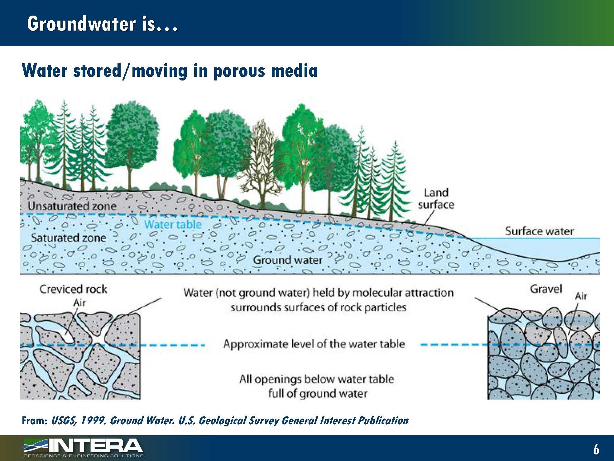 Groundwater is water stored or moving in porous media in the saturated part of the subsurface; water in the vadose zone (or unsaturated zone) is technically not groundwater; it’s held by capillarity and follows similar physical laws.
Groundwater is part of the water cycle. All groundwater starts as surface water and arguably ends as surface water; Mr. Singh said that this is important because when we start talking about the physical processes and how we set up models and boundary conditions, one really needs to keep in mind that the groundwater part of the basin is part of a larger system – more regional or global system. In fact, sometimes it becomes a challenge in how we define the boundary between groundwater and surface water.
 Groundwater is connected to surface water; the graphic shows the relationship. In a gaining stream, groundwater discharges to the surface water body. In a losing stream, groundwater is recharged, depending on the relative head gradient between the water in the surface water body and the water table. Oftentimes, groundwater can become disconnected from a surface water body but still get some recharge if there’s water in that surface water body.
“It is important to keep this in mind when we start thinking about how to set up the model and what kind of processes and boundary conditions we want to simulate,” Dr. Singh said.
 Groundwater can be either confined or unconfined; confined and unconfined groundwater behaves in different ways. Confined groundwater is found in settings where the groundwater is in a pressurized pore space; typically, this happens when the recharge area is at a higher elevation than the area where you might be pumping or doing an evaluation, he said. Groundwater can be unconfined, and in that setting, it’s exposed to atmospheric pressure.
Groundwater follows the laws of physics, and over the last hundred years or so, a lot of understanding has been developed on what laws of physics groundwater follow. Some of the fundamental laws are conservation of mass and volume, where inflows minus outflows change storage and conservation of momentum (or Darcy’s Law). If groundwater is at different elevations, the flow through that system depends on the head gradient as well as the hydraulic connectivity. The groundwater velocity through the aquifer depends on the flow as well as the porosity.


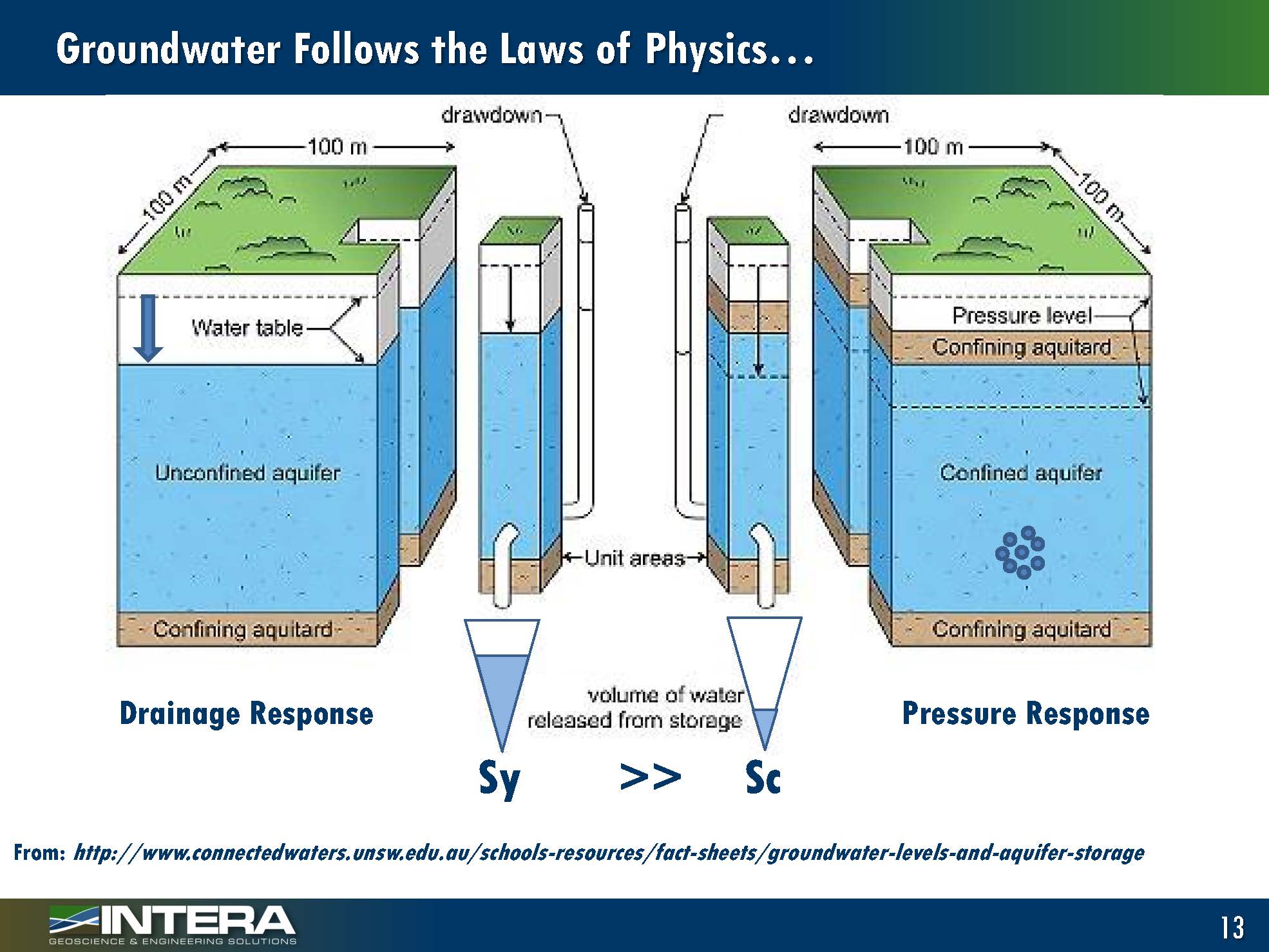 Dr. Singh also noted that confined and unconfined groundwater have very different storage properties. Unconfined groundwater displays a drainage response, so the amount of water you get when the water table decreases is driven by the drainage characteristics of the porous medium. However, confined aquifers display a pressure response where the amount of water you get when the head in the confined aquifer decreases depends on the structural properties, such as how much the matrix itself compresses, so in general, you have a much higher yield of groundwater from unconfined systems and more groundwater produced for lower levels of drawdown as compared to confined aquifers.
WHAT IS A GROUNDWATER MODEL?
A groundwater model is essentially a representation of a physical groundwater system. This representation can be conceptual and may be depicted pictorially. Once that is done, it can be represented mathematically. So a groundwater model can be a mathematical representation of a physical groundwater system, and in fact, Darcy’s Law is arguably a mathematical model that is used to represent the flow system in groundwater aquifers, Dr. Singh said.
 The model could be an analytical representation of a physical groundwater system, which means we have a mathematical equation that we can solve. It could be a numerical representation, in which case we define our groundwater system, split it into small pieces, and solve the mathematical equation using numerical methods.
“In any case, whatever kind of groundwater model we are dealing with, we start with reality, and that is our best understanding of the subsurface truth,” said Dr. Singh. “We abstract it into a conceptual model where we try to represent the key processes and the key hydrogeologic characteristics of the real groundwater system. This conceptual model can then be represented as a mathematical model, so the processes we have defined in the conceptual model need to be represented using mathematical terms … There are standard equations, standard solvers that we can use to represent our conceptual model in a mathematical setting. Once we have the mathematical model, we can solve it or simulate it using a numerical setting, and in some cases analytical setting.”
The groundwater model is an abstraction or an approximation of the real system; the level of abstraction or approximation really depends on the purpose of the model. So in developing the groundwater model, we need to carefully consider what the groundwater model is going to be used for, what the key processes are, and the appropriate model scale that needs to be built to be consistent with modeling goals and purposes.
“To give you an example, a model that’s constructed to compute regional budgets which is likely fairly coarse, may not be appropriate to predict seawater intrusion, which is a highly localized process driven by local gradients and density effects,” said Dr. Singh. “So a model at a regional scale may do very well in simulating the overall water budget of your basin, but may not be appropriate to predict local flow systems or local head responses.”
‘All models are wrong; some are useful’ is a bit of a cliché, but Dr. Singh reads the term ‘wrong’ to refer to the process of abstraction or approximation. “So all models are approximations, but some approximations are useful,” he said. “It’s up to you as a modeler is to ensure that the abstraction and approximation is commensurate with the purpose of the model and the decision-making process that the model is driving.”
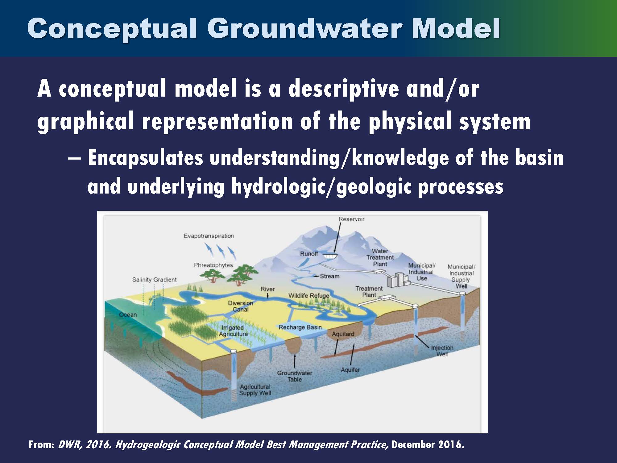 A conceptual model can be a descriptive or a graphical representation of the physical system. Its purpose is to encapsulate the understanding or knowledge of the basin and the underlying hydrologic or geologic processes. Developing the conceptual model can sometimes be very complex, and oftentimes it’s where the most time is spent because you’re dealing with the lack of understanding and developing an understanding from data.
“The conceptualization is a very, very important part of the modeling process and one needs to be very deliberate, very thoughtful, and you need to make sure that you’re accounting for the best available data and science that’s out there,” said Dr. Singh.
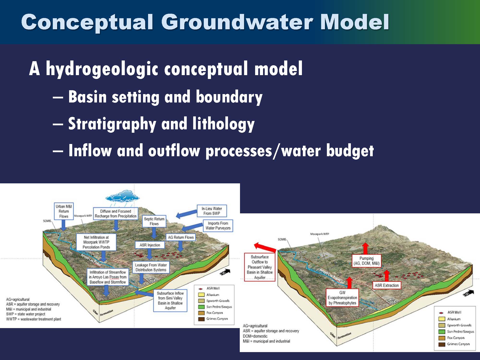 A hydrogeologic model, a subset of a conceptual model, typically defines the basin setting and boundary stratigraphy, lithology, and the key inflow and outflow processes of a water budget. The slide shows an example where all the key inflow and outflow processes for the basin have been identified, and the stratigraphy has been defined so where the water might be going in or coming out from is known. This is really the start of the hydrogeologic conceptual model base. Once the conceptual model is developed, it is then translated into mathematical equations that describe and, most importantly, help to predict the response of the groundwater system.
“The mathematical equations are important because if you go back to a conceptual model, the conceptual model describes your groundwater system, but on its own, it doesn’t really give you the ability to predict anything in the future,” said Dr. Singh. “You have to build these mathematical relationships between dependent and independent variables of the groundwater system to be able to predict response to future stresses.”
The slide shows the transient groundwater flow equation, which basically says that the flow is dependent on the connectivity and the head gradient and that the change in flow in any direction is equal to the change in storage, thus sources or sinks. If the storage component is eliminated, then it is a steady-state equation where there is no change in storage, and the change in flow in any particular equation is equated to the sources or sinks in the groundwater system.


In certain cases, the mathematical equation can be directly solved. “For example, this is your classic Theis equation where we know the transient drawdown response to pumping at a location,” Dr. Singh said. “There are several analytical solutions for different boundary conditions and different assumptions for the processes underlying the groundwater aquifer, and so these analytical solutions are exact in that they don’t rely on numerical discretization; you just solve the mathematical equation, and you have an exact answer at any given point in space or time.”
 However, groundwater systems are typically more complex than represented in analytical solutions. The mathematical equations have to be solved numerically and to do that, the spatial domain is divided into smaller subunits. Dr. Singh explained that there are several ways to do this, such as finite difference, finite element, finite volume – but the main idea is to take the overall groundwater system and split that into smaller subunits, which you assume to have uniform properties. The time domain is split into small timesteps, so you assume that things remain constant within each timestep. So space and time are now divided into subunits, and the mathematical equations apply to each subunit in space and time, and then you solve the system of equations. To do so, you will need to define initial and boundary conditions.
WHY USE GROUNDWATER MODELS?
Groundwater models are really decision support tools.
There are four fundamental uses of groundwater models:
To understand and characterize a groundwater system: Groundwater models are our best understanding of how the aquifer works.
To predict how the hydrogeologic system responds to future stresses or changes.
To quantify the uncertainty as well as the certainty in our current understanding and future predictions. “For example, you can use groundwater models to say, here is how sure I am that water levels are going to change by 20 feet if I pump 500 GPM from this location, or this is the uncertainty in that prediction because, in a groundwater model, you can start looking at different sources of uncertainty and running them into your model predictions to assess the range of different outcomes.”
To decide where additional data or field testing is needed to reduce the underlying uncertainty and make the predictions more robust.
The Best Management Practices for Sustainable Groundwater Management released by the Department of Water Resources in 2016 listed several uses for groundwater models:
- to improve hydrogeologic understanding;
- to simulate the aquifer;
- to calculate and verify water budget components;
- to predict impacts of hydrological or groundwater management changes;
- to assess sensitivity and uncertainty to guide data collection and risk-based decision making; and
- to visualize and communicate aquifer behavior to stakeholders.
Ultimately, groundwater models become the repository for groundwater information, data, and knowledge as the model is built and refined over time with more data, new information, and knowledge.
HOW ARE GROUNDWATER MODELS DEVELOPED?
Overview
The schematic shows the overall process. The first step is to define the model objectives because everything is linked to what the model is going to be used for.  Then based on those modeling objectives, you collect and compile data. There may be a requirement to go out in the field and collect more data if there is insufficient data to build the model. Based on the data and the analysis, you start putting together your conceptual model, which is the pictorial or graphical understanding of the processes and the geologic characteristics of the basin. Once the conceptual model has been developed, the model design phase begins.
The model is designed and then calibrating the model, which entails changing the model properties and boundary conditions to replicate the past based on observed records. Calibration can be steady-state or transient. Steady-state would be in cases where a basin under certain conditions didn’t change a lot, such as during predevelopment conditions; transient calibration would account for changing water levels and changing flows in your basin.
Once the model is calibrated, the model is verified by running it through a period of record that was not used for calibration purposes. Once the model has been calibrated and verified, you get into the prediction mode. Now you start running your model with changes to boundary conditions or stresses in the future to assess how the basin will respond to those changes. There is also reporting and integration into the overall water management strategies.
Model grid
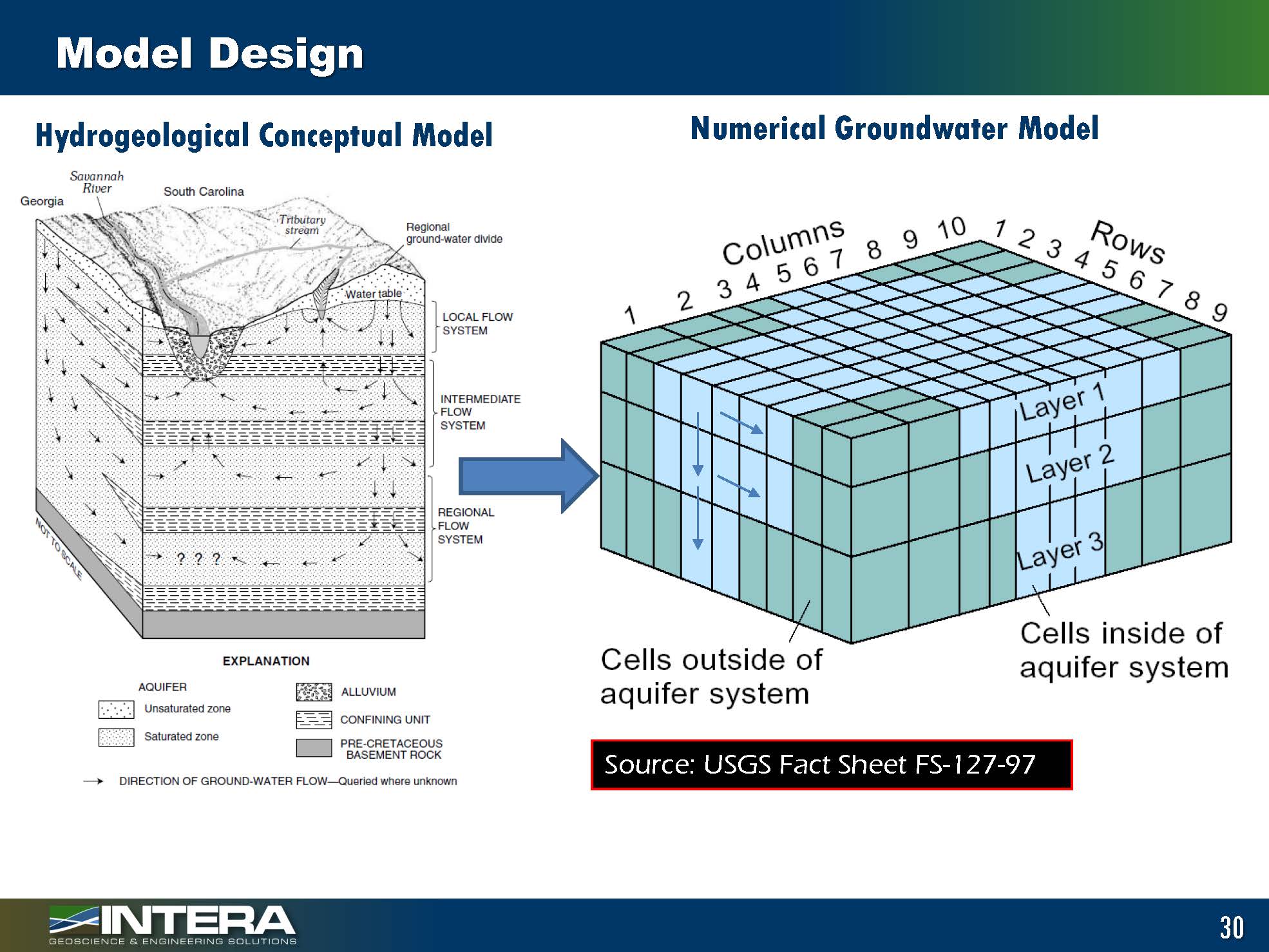 The model design phase itself starts with the conceptual model. Everything has to be linked to the conceptual model, Dr. Singh said. So the conceptual model is broken down into smaller and smaller pieces to represent the aquifer as a series of grids and layers with some of these layers representing boundaries and some of these cells represent the actual aquifer system.
“The model design phase really needs to be balanced because the model grid really is the smallest scale at which the model solution will be computed, so the scale has to be chosen such that it is consistent with model use,” said Dr. Singh. “Coarser resolutions may be okay for a model meant for water budget calculations; finer resolutions will be needed where local gradients need to be simulated, so this process of design, this process of defining and discretizing the model domain really depends on what you’re going to be using the model for. So if you’re looking at groundwater-surface water interactions or wellfield assessments or fate and transport, then you need a finer resolution model because those are all processes that are driven by local gradients at a fine scale.”
“Overall, what you’re trying to achieve is a balance between computation efficiency so the higher resolution the model becomes, the more computation expensive it becomes with model accuracy, so you want to have the coarsest model which gives you the most accurate results for the decisions you’re trying to make.”
Boundary conditions
 Once the model grid has been defined, the next step is to define the boundary conditions which represent the interaction of the model domain with the environment. This is where water is either coming in or leaving. There are three basic types of boundary conditions: the specified head (type 1), specified flux (type 2), or head-dependent fluxes or mixed (type 3).
“The determination of which boundary to use is part of the art and science of groundwater modeling,” said Dr. Singh. “Ideally, you want to use hydraulic or geologic boundaries, so if there are geologic outcrops that represent no flows in your basin, those boundaries should be chosen as no-flow boundaries; if there are groundwater divides or flow directions that could be used to identify interfaces where you don’t expect water to flow across, those again would be no flows.”
Artificial boundaries can be defined. If there is water level data in the part of the basin, it can be used to set up artificial boundaries, which are specified head boundaries but not real geologic or hydrogeologic boundaries. Dr. Singh cautioned that you need to be careful and place them far enough away from the area you want to evaluate so that the boundaries do not affect model output.
“This is where the concept of distance boundaries arises, so in all cases, you want to make sure that there is minimal interaction or interference between your boundaries and the area of interest that you’re going to be changing stresses and evaluating responses to.”
Specified head
In specified head boundaries, the head remains constant. Water is simulated as moving in or out of the groundwater at a rate sufficient to maintain the specified head. Specified head boundaries typically represent a boundary of the body of water of where there is a known fixed elevation.
With this type of boundary, it is important to ensure that any extraction or recharge within the model domain does not interact with that boundary, Dr. Singh said.


For example, the slide on the left shows a specified head boundary; there is a regional gradient, so water is flowing from west to east. If a well is placed next to that boundary, the well will induce more water to flow in from that boundary, which can end up acting as an infinite source of water, which is not realistic.
“So you have to be very careful when you use these specified head boundaries and make sure that you don’t have any changes in model stresses happening along those boundaries that might interfere or influence the boundary itself,” said Dr. Singh.
Specified flux boundaries
 In specified flux boundaries, the rate of water moving into or out of the groundwater is specified. Specified flux boundaries are used when boundary fluxes are independently estimated, typically recharge, underflows, and pumping. No flow is a special type of specified flux boundary where there is no flow.
“I prefer specified flux boundaries whenever possible because they constrain the overall water budget,” said Dr. Singh. “Obviously, there is no potential for infinite sources or sinks, so your overall water budget is defined. Oftentimes in the process of calibration, you might encounter that you need more water or less water, and that forces you to actually go back and revisit the conceptual model and revise your understanding of the overall basin setting and the inflow and outflow processes.”
Head dependent flux boundaries
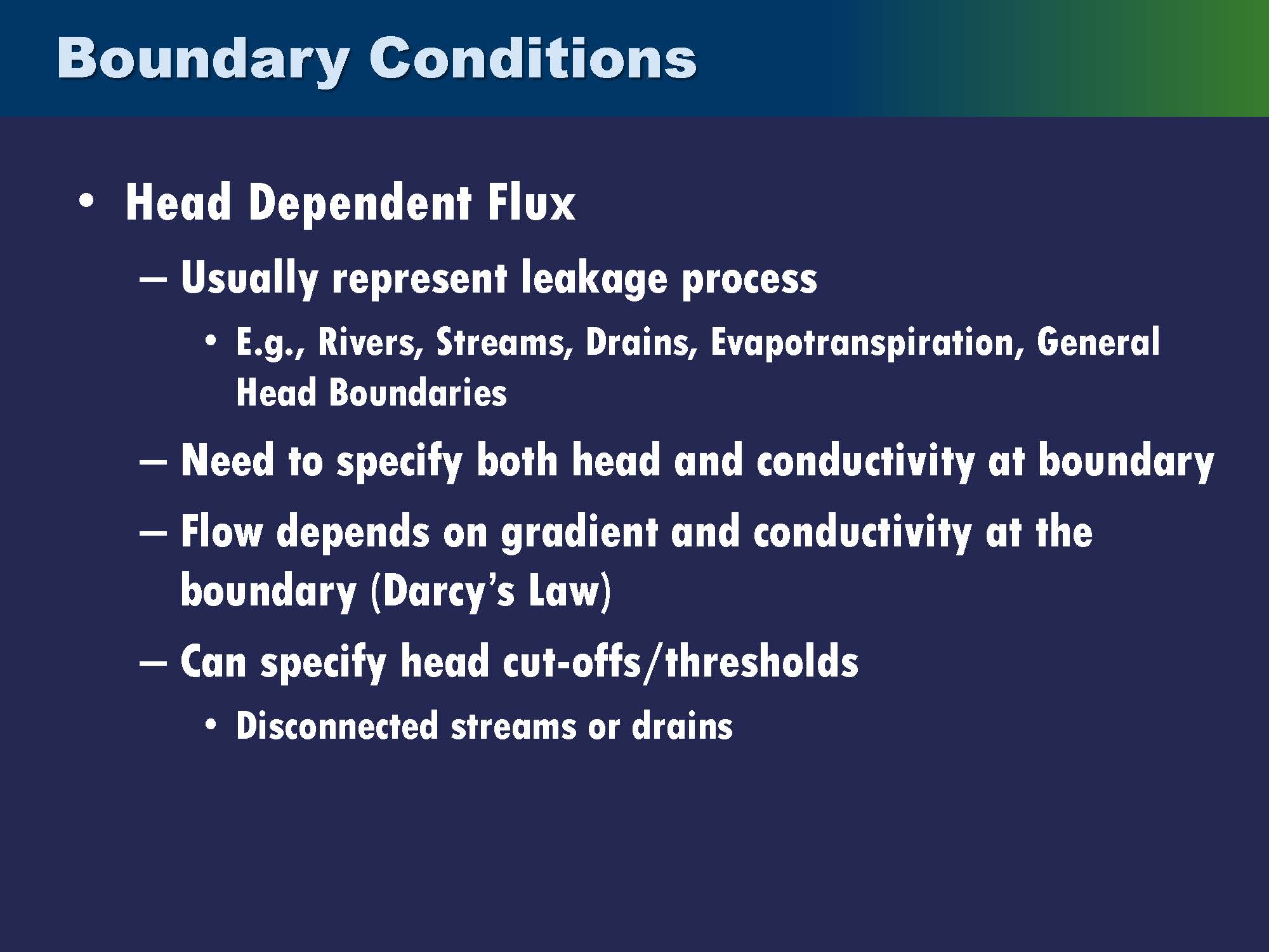 In head-dependent flux boundaries, the rate of flow from the boundary into or out of the groundwater varies in response to changes in the head in the boundary cell. They usually represent leakage processes. These are the boundary conditions that are the most flexible, so they are used for rivers, streams, drains, evapotranspiration, and general head boundaries.
“In these cases, you need to specify both the head at the boundary as well as a boundary conductivity,” said Dr. Singh. “What the model does is it uses Darcy’s Law to calculate the flow based on the gradient between the head that you specified at the boundary and the head in the next adjacent model cell, using the connectivity of the boundary itself.”
Head dependent flux boundaries are flexible; you can specify cutoffs and thresholds where there would be flow would be constrained or no flow, such as in a drain where if the head falls below the elevation of the drain, there would be no outflow.
“Head dependent flux boundaries give you a lot of flexibility, but similar to specified head boundaries, you have to be very careful how you use them and to make sure that they are consistent with the conceptual model and the water budget that you have estimated for the basin,” said Dr. Singh.
 Groundwater-surface water interactions are best represented with a head-dependent flux boundary. Ideally, the head of the stage in the river or stream would be based on flow in that channel, so there would be a surface water routing element in the model that defines the flow, which leads to the stage, and then is coupled with the groundwater system. Based on the gradient between the stage and the groundwater table, you could either have groundwater losses or gains, or the water table itself might get disconnected and just get constant recharge.
“This is an example where you have a threshold effect where once the water table falls below the bottom of your stream bed or river bed, you essentially have constant recharge into the groundwater table from the stream bed,” he said.
Other model parameters and inputs
There are other parameters to be defined in addition to model boundaries, such as the stratigraphy. There are hydraulic parameters such as connectivity and storage coefficients where the hydraulic connectivity is really the driver of the flow system, and the storage coefficients of specific yields are how the basin responds in time to different stresses.
Once the parameters and boundary conditions have been specified, the last step is to specify the initial heads.
“For a transient model, you need to start from somewhere, so you define those specific heads, and you run your model to calculate your flows and your heads in time,” he said.
Model Calibration
Next, the model must be calibrated. For a groundwater model to be used in any predictive role, it must be demonstrated that the model can successfully simulate observed aquifer behavior.
The model calibration process involves matching observed and simulated data by adjusting independent variables, such as hydraulic connectivity, storativity, or recharge, and running the model repeatedly until the computed solution matches observed values within an acceptable level of accuracy. Oftentimes, the boundary conditions might have to be adjusted or the basin stratigraphy depending on local water levels or where you’re not matching observed water level or flow data.
 “You really need to make sure the calibration includes all relevant data put into model predictions, so if you’re interested inflows and gradients, make sure that you use flows and gradients to calibrate your model,” said Dr. Singh. “So use hydraulic head data from the basin, but if you have independent estimates of flows or streamflow measurements or stream gains or loss studies, use those to constrain the simulated flows from the model. Oftentimes, using vertical and lateral gradients to constrain calibration is much more powerful than just matching hydraulic head measurements.”
The calibration data should really cover the range of variability of transience that you expect in the predictive domain.
“For example, if you’ve calibrated your model to a period with relatively high water levels, you should be very careful using that model to predict responses during drought conditions,” he said. “The model has been trained within a certain setting, and ideally, you want the training of the model to be consistent with how you’re going to test the model or use it in the predictive setting.”
Dr. Singh noted that the other confounding thing that modelers run into, especially with groundwater models, is that groundwater model calibration is a non-unique process, which means that multiple parameter combinations, such as combinations of recharge and conductivity, can yield similar calibration results.
“With this non-uniqueness, uncertainty is introduced in the underlying calibration process, so it becomes really important to incorporate as much prior data we have for model parameters,” he said. “If we know that certain model conductivities are representative of certain hydrologic settings, you want to make sure that the calibrated parameters are consistent with that. So as a modeler, you have to constantly assess the plausibility of results – looking at the flow field and the conductivity distribution to make sure that it’s consistent with our conceptualization, the basin setting, and the deposition setting that your aquifer corresponds to.”
“Ultimately, because of the non-uniqueness and because of data gaps in the model calibration process, you have to make sure that the calibrated parameters, as well as the water budget, are consistent with your conceptual model,” he said.
Verification
Once the model has been calibrated, it must be verified. Typically, this is done by using historical data not used for calibration and running the model through that time period to make sure the model can represent data that wasn’t used during calibration. Once the process of verification is complete, you can run the forward model and look at predictions based on future changes to the basin stresses.


“The basis for the accuracy of your prediction really depends on the ability of the model processes,” Dr. Singh said. “You have to make sure that the model is calibrated and has been built with the processes that you need to test during the predictive time frame. It depends on the accuracy of the data that you have, the knowledge of hydraulic conditions, and the reliability of the estimates of the system stresses itself. So, for example, if you’re running simulations with future pumping or future recharge, then obviously the predictive accuracy will depend on how accurate our projections of recharge and pumping are.”
HOW CAN GROUNDWATER MODELS BE USED?
Once the groundwater model has been developed, calibrated, and verified, it can then be used to answer different types of questions.
Dr. Singh said there are five hierarchies or levels of questions that groundwater models can be used to answer:
On the broadest scale, a model could answer questions related to regional flows, such as what is the current or future water budget for my groundwater basin? Or how much recharge does my basin get from the river?
The next level would be regional water levels, answering questions such as, what will groundwater levels in my basin be in ten years? A model could tell you about the spatial distribution of water levels, such as how will basin levels respond to recharge or a wellfield project? Based on the question asked, there would be an appropriate scale that you set up the model for, he said.
Higher-resolution models can answer questions related to local flows, such as how much water does my wellfield pull from the river? Where is the water from my wellfield going? What are the sources for seawater intrusion, and how can we prevent seawater intrusion from happening? Will my wellfield capture the contaminant flows? These are all questions related to the local flow system, so a higher resolution model with better calibration and more localized data is needed to answer these questions reliably.
Higher-resolution models can also answer questions about local water levels, such as, are there pumping interferences between my wellfields? How much drawdown should I expect in my well? Dr. Singh noted this tricky because oftentimes, when using numerical models, they don’t have the requisite resolution to calculate drawdown within the well. Will pumping cause subsidence in the basin, and if so, where and how much? In this case, local groundwater levels are important, but you also need to ensure that you represented the physical processes for subsidence.
There are complex multi-level questions like, what are the most hydrologically conducive areas for my wellfields and recharge projects? To answer this, you might have to look at regional and local effects iteratively and optimize where you’re putting your wellfields or recharge project to reach some basin-scale objectives. At an even higher level, what management actions should I implement to ensure sustainable water levels in the future?
These complex questions need to be broken down into corresponding regional or local flow or water level questions and then answer iteratively and consecutively to get to the final answer.
 “The ability of the model to answer these questions really depends on the processes that are simulated because a model that does not simulate the processes you are interested in predicting cannot answer the question that you ask,” said Dr. Singh. “So if you haven’t adequately simulated groundwater-surface water interactions, you will not be able to answer questions related to surface water capture by wells.”
“The model needs to have the appropriate boundary conditions, so if you’re using specified heads or head-dependent boundaries, be very careful using those models for water budget analysis,” he continued. “You need to make sure that you have independent estimates of water budgets to verify the fluxes that you’re seeing across those boundaries. A model without coastal boundary cannot be used to assess seawater intrusion. The scale, resolution, data availability, and finally the level of calibration are key considerations when you are looking at the ability of the model to answer some of these questions.”
CASE STUDIES
Dr. Singh then provided some case studies.
Case study #1: Santa Monica Basin Water Budget
 The first case study is a water budget analysis for the Santa Monica Basin. The model used was the Regional USGS LA Basin Model, a regional model covering the entire Los Angeles coastal basin.
This is important because the Santa Monica basin is not isolated; there are underflows from adjacent basins that need to be simulated. In this case, a regional model is more appropriate than a local model because it includes those underflows.
The model was fairly coarse with about an eighth-mile grid that includes all the physical processes at the regional scale and boundary conditions that are far enough away from the Santa Monica basin for the water budget, managed recharge, and extraction to be evaluated.
“With this regional model, we can assess localized water budgets by going in and essentially piecing out the water budget for the subbasin itself,” said Dr. Singh. “So we’re running the regional model but extracting the results at the basin scale.”
He presented the sample results, noting that they were able to look at recharge and discharge within the Santa Monica Basin as well as the underflows to adjacent basins, which would be hard to assess if the model was only local for the Santa Monica basin and had artificial boundaries or specified head boundaries on the edges.


Case study #2: Feasibility Assessment and Preliminary Design of Wellfields in the LA Basin
Another case study was evaluating the feasibility and developing the preliminary design of wellfields in the Los Angeles Basin. In this case, the regional model was too coarse for wellfield scale analysis. So they started with the regional model and then built a high-resolution model based on boundary conditions linked to the regional model. Still, the local geology was based on basin field-scale data.
The LA DWP was interested in siting, feasibility, and preliminary designs for wellfields; there were six locations under consideration. The region model was a four-layer model that they broke up into thirteen layers to correspond with the aquifers and aquitards in the basin.


They developed a high-resolution model with grids at 10 feet by 10 feet because they were interested in calculating drawdowns of each well to see there would be dewatering issues or if they needed to screen the well to pump at certain rates without running into water levels below the screening interval. Where to screen the well and what aquifer it would be in was a key question in terms of feasibility and project costs.


“Using this model, we were then able to come up with the capacity of the wellfields as well as the drawdowns and the recommended screen intervals,” said Dr. Singh. “We were able to use this localized model to look at subregional drawdowns and also drawdown at the well scale within the well bore and accounted for efficiency losses.”
Case study #3: Modeling GW/SW Interactions with the MODFLOW SFR2 Package
The final case study is one where they modeled groundwater-surface water interactions with the MODFLOW package, which is the USGS’s modular hydrologic model. MODFLOW is considered an international standard for simulating and predicting groundwater conditions and groundwater/surface-water interactions.
They used MODFLOW to evaluate an arroyo in the Las Posas Basin in Ventura County. The arroyo itself is highly transient and characterized by a braided stream channel, a variable channel width, and no permanent river banks, so they used the SFR 2 package to route flows and simulate surface water-groundwater interactions. The arroyo itself was delineated by using high resolution, 10 feet by 10 feet LIDAR data; the inflows were calculated based on data for wastewater treatment plant discharges and upstream flow gauges. The stream itself was broken into multiple channels because the flow gradient curve relationships were different in different parts of the basin based on the topography and local geology.
Each of these segments then had its own flow depth and flow width relationship with fairly high-resolution gridding.
 “This is the same stretch of the river under strong flow conditions and dry conditions, and as you can see, the arroyo itself changes drastically based on flow conditions, so to be able to simulate this, we had to have a dynamic surface water-groundwater interaction package and account for all the hydrologic processes and the dynamism in the underlying system,” Dr. Singh said.
So depending on the location within the basin, the channel width changes with different flow regimes, and they were able to calibrate the model to replicate the flow conditions. The model was calibrated not just to water levels but also to streamflows and vertical and lateral gradients.
“This is where the power of multi-criteria calibration became very important because we were really interested in those small scale gradients between the stage in the arroyo and the groundwater table itself,” he said.
MODEL UNCERTAINTY
Lastly, even if the model has been integrated and calibrated to all available data, there remain uncertainties: Conceptual uncertainties related to basin understanding, stratigraphy and boundary conditions, parametric uncertainty due to non-uniqueness, data gaps, calibration errors, and residuals, as well as the data that the model is calibrating to, could have measurement errors itself.
“That uncertainty is fundamental, and it’s up to the modeler to make sure that the model is used in the appropriate context and the results are presented in the appropriate setting to be able to communicate the uncertainties in the model,” said Dr. Singh.
IN SUMMARY …
“In summary, groundwater models are conceptual, mathematical, or numerical representations of the physical groundwater system,” said Dr. Singh. “The level of representation of abstraction really depends on what the model needs to be used for. The models should be developed based on the best available data and understanding of hydrogeologic processes, and the model representation and calibration should always be linked to the conceptual model as well as what the model is going to be used for.”
“Groundwater models can be used to answer questions related to regional and local flows and water levels,” he continued. “The ability of the model to answer such questions depends on the processes that you’re simulating, boundary conditions, scale, and the level of calibration. Finally, all models are inherently uncertain and have limitations, and so it’s up to you to use them judiciously and carefully.”
QUESTIONS & ANSWERS
Would you comment on the relative merits of finite-difference versus finite elements, and when might you use one or the other?
“In general, the finite element scheme gives you the most flexibility when it comes to representing the physical systems, so if you have complicated or highly irregular boundaries or complex stratigraphy, then finite element schemes will give you the maximum flexibility,” said Dr. Singh. “With finite difference, you are forced to use essentially a block approach to representing your domain as well as your boundaries. On the flip side of finite element schemes and to be mathematically more complex, setting up the appropriate finite element functions and having the right solvers can sometimes be challenging. I’ve used both fairly effectively, but typically finite difference models are easy to set up, but again, if you have a very complex structure and stratigraphy, then finite element schemes would be more appropriate.”
Question: I’ve read from reports from the Texas Water Development Board, groundwater availability models, for example, that it usually takes a long time to develop and calibrate a regional groundwater model. Will changes within the area during the development become important on a large scale?
“No groundwater model is ever complete,” Dr. Singh said. “Even if you don’t have changes to your basin, you’re collecting more data, and you’re refining your understanding of the basin, but certainly if you have management changes in your basin, you would want to update the model and integrate them into the model stresses that you’re simulating. It’s an ongoing process; it’s an iterative process. You have a threshold in time when you say here is where we are going to stop the calibration period, then you went for some time, collected more data, assess changes that are happening in your basin, and then update the model subsequently.”
Question: How do we consider the uncertainties in the model in our decision-making process?
“I don’t know if I have enough time to really do justice to the question,” said Dr. Singh. “There are multiple levels of uncertainties in the groundwater model itself. There is conceptual uncertainty; there’s parametric uncertainty, calibration errors, as well as measurement errors. In general, the process you need to follow is first, you need to characterize and quantify the underlying uncertainty, so if, for example, you don’t have a good handle on stratigraphy, we may come up with alternative model structures so that certain model errors could be higher or lower within the range of uncertainty for that structure. Or if we have uncertainty with respect to certain fluxes, we would come up with a range of those fluxes. Then you essentially have to go through a process of looking at multiple alternative models with the range of uncertainty when it comes to either the conceptual model or parametric uncertainty as well.”
-
- Modeling BMP (Department of Water Resources)
- Projecting Forward: A Framework for Groundwater Model Development under SGMA (Water in the West)
- Adjudicating Groundwater: A Judge’s Guide to Understanding Groundwater and Modeling (The National Judicial College)
- Integrated Hydrologic Model Development and Evaluation for Non-Modelers, article at Maven’s Notebook

